For a farmer considering a cover crop, a change in tillage, or livestock integration, several questions arrive together. What will it do for the soil? How will the crop respond? What will it cost, and what might it save?
Jonathan Lundgren and colleagues brought those questions into the same study. Across 210 farms in 15 U.S. states and two Canadian provinces, they measured soil carbon and biological communities alongside farm production and economics. Their August 2026 paper examines how those outcomes vary across established management systems. [1]
The supplementary figures and public data add a useful finding for farm planning: fields with similar practice scores often had very different outcomes. Looking at those differences can help farmers choose what to measure before adding another practice. [4][5]
Looking at the farm as a system
The farms were sampled in 2022 and 2023, after their management systems had been in place for at least four years. The researchers scored eight practices: no tillage, cover crops, organic amendments or manure, grazing, and the absence of synthetic fertilizer, herbicides, insecticides, and fungicides. In the main classification, farms using four or more practices were considered regenerative. [1]
The score counts how many of those practices were present and gives each equal weight. The same score can represent different combinations: one point might mean a cover crop, manure, or the absence of an insecticide. When choosing a change, consider its rate, timing, duration and implementation alongside the count. [1]
These established operations differed in soils, locations, crops, histories and management experience. The paper’s carbon analysis accounted for rainfall and clay content. Following the same farms through management changes would help explain how their outcomes develop over time. [1]
The team collected soil cores down to 60 centimeters—about 24 inches—and compared equal masses of soil to account for differences in density. They also measured microbial communities, non-crop plants, invertebrates, and birds. There were 181 usable management scores; individual analyses used smaller subsets, including 80 farms for bird surveys and 98 fields for the main corn, soybean, and wheat yield comparisons. [1]
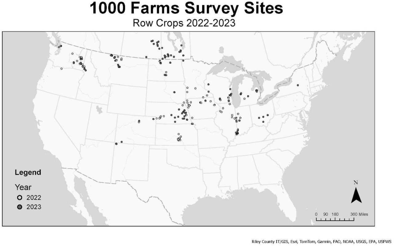
How closely do the sampled regions match your crop, rainfall, growing season and soils? Those comparisons can help identify which results are most relevant and where a local trial or an adviser’s experience would be useful.
A larger carbon store, with substantial variation among fields
The overall fitted relationship points toward more total carbon at higher management scores. Using Table 1’s printed equation, y = 4.19x + 74.82, SHE calculates 74.82 Mg C/ha at score zero and 104.15 Mg C/ha at score seven. The fitted difference is 29.33 Mg C/ha, or 39.2%—about 13.1 U.S. tons of carbon per acre. [1]
The observed group averages in Table 1 were 67.93 Mg C/ha (30.3 U.S. tons C/acre) at score zero and 96.91 Mg C/ha (43.2 U.S. tons C/acre) at score seven. The figure shows those sampled averages; the equation summarizes the overall fitted relationship. A U.S. ton is 2,000 pounds. These are carbon stocks in the soil profile compared. [1]
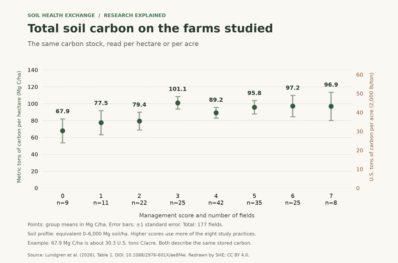
Score three had Table 1’s highest observed mean total carbon: 101.1 Mg C/ha across 25 fields, compared with 96.9 Mg C/ha across eight fields at score seven. Higher practice counts did not consistently correspond to higher group averages. [1]
Practice count alone explained a small share of the differences among fields. Table 1 reports R² = 0.03 for total carbon and 0.02 for organic carbon in its simple straight-line fits. SHE’s analysis of 177 fields gave similar results: 2.4% of the variation in total carbon stock and 1.6% in organic carbon stock. These describe the score alone; the authors’ models that also considered soil and rainfall address a broader question. [1][5]
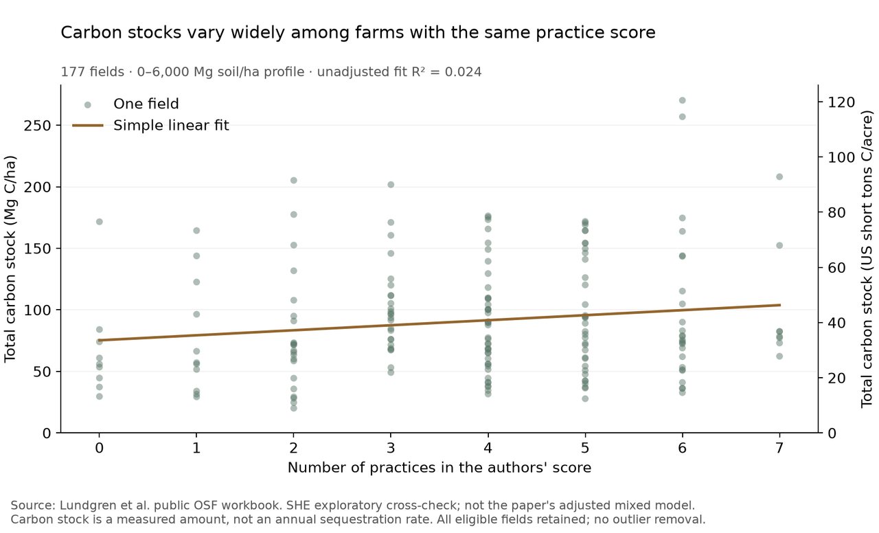
In SHE’s separate workbook analysis, six of the eight score-seven fields fall below the fitted line; two high-carbon fields lift the group mean to 102.0 Mg C/ha, compared with a median of 80.3 Mg C/ha. [5]
For your farm, pair the practice list with soil texture, rainfall, previous management and repeated measurements. The individual fields, mean and median together show why a farm with the same score may still have a different carbon store.
Ask which carbon fraction changed, and where
The study measured organic carbon, associated with once-living material, and inorganic carbon, including carbonates. The supplementary results show a management-score association with organic carbon in shallower layers, while the lower 3,000–6,000 Mg soil/ha stratum has no clear association (P = 0.27). Equivalent soil mass compares the same amount of soil across fields; its boundaries can fall at different depths where soil density differs. [1][4]
When planning a follow-up sample, record the depth or equivalent soil mass, the laboratory method, and whether the result is total, organic or inorganic carbon. Keeping those details consistent makes a later comparison more useful.
More life above and below ground
Higher-scoring fields had more microbial biomass, more non-crop plant species, and greater invertebrate abundance and species richness. The authors’ fitted endpoint comparisons estimated about 66% more total microbial biomass and 181% more fungal biomass at score seven than at the score-zero baseline. [1][4]
Microbial biomass was estimated using phospholipid fatty acid analysis, or PLFA: lipid markers that characterize broad groups of soil organisms. For non-crop plants, the supplementary fitted line rises from about 0.16 to 2.75 species per 0.1 m² between scores zero and seven—roughly a one-square-foot sampling area. These are fitted averages for small sampling quadrats. The identity of the plants and when they grow help determine their value and management demands. [1][4]
Bird surveys found a positive relationship between score and bird species richness. For the number of individual birds, the main text reports no increase, while Figure S4 reports a positive association (P = 0.004) after removing one outlier. The different results call for clarification of the analysis. [1][4]
The carbon fraction matters when connecting bird counts to soil measurements. In supplementary Table S2, bird abundance was associated with inorganic carbon across the three cumulative profiles, but not with organic carbon (P = 0.75–0.93). Location and environmental conditions are useful questions to investigate here. For farm observations, record both bird numbers and species, with consistent timing and survey effort. [4]
Choose a biological measurement that answers your question
Table S1 shows how closely several indicators tracked total soil carbon in this sample; a higher R² indicates a closer relationship. Using an indicator to estimate carbon stocks requires calibration and validation for the soils and conditions where it will be used. [4]
Different measurements capture different parts of the system
| Measurement | Reported R² with total carbon | Useful interpretation |
|---|---|---|
| PLFA group-diversity index | 0.29 | Describes the relative balance among broad lipid-based groups; species diversity and ecosystem function are separate questions. |
| Fungal biomass | 0.18 | Adds information about the fungal component of the soil community. |
| Total microbial biomass | 0.17 | Estimates the size of the living microbial pool measured by PLFA. |
| Total ground cover | 0.03 | Directly describes surface protection, even where its relationship with total carbon is weak. |
Do gains level off as the practice score increases?
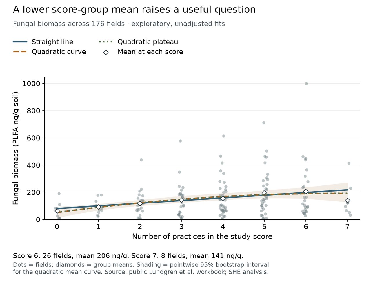
SHE compared straight-line, quadratic and quadratic-plateau fits for eight outcomes in the public workbook, with 166–177 fields available for each. A quadratic can rise and fall; a plateau rises and then levels off. Each field contributed one average to the fit. [5]
Fungal biomass illustrates the pattern. The observed mean was 206 PLFA ng/g soil at score six across 26 fields, compared with 141 ng/g at score seven across eight fields. The apparent quadratic peak near score 6.8 moved outside the observed range when the score-seven fields were omitted. About 52% of 1,000 field-resampling runs produced a downward-opening peak within scores zero to seven. That sensitivity leaves the location of a peak unresolved. [5]
Responses differed among outcomes
| Outcome | What the exploratory comparison found |
|---|---|
| Organic carbon | Curved fits added essentially no explanatory power and predicted held-out fields slightly worse than a straight line. |
| Ground cover | A possible plateau around scores 3–4 was highly uncertain. The plateau reduced held-out prediction error by only about 0.3%. |
| Fungal biomass | The high-score dip depended strongly on a small endpoint group; a stable peak was not resolved. |
| Non-crop plant richness | The fitted curve continued upward toward score seven rather than showing an upper-score decline. |
These curves help identify measurements to follow on a farm, but a dependable stopping score remains unresolved. Testing which practices add value would require their individual records and comparisons within similar soils, climates and cropping systems. The public workbook supplies the total score. For a field decision now, start with the function the next practice could add. [5]
Build a combination around the functions your field needs
NRCS soil-health guidance provides a useful way to think about complementary practices. Residue and cover crops both protect the surface, while a living cover crop can extend root activity and capture nutrients between cash crops. Manure can supply organic material and nutrients where the nutrient budget supports it. These functions overlap, and their value depends on species, timing, rates and existing conditions. [6][7][8]
Match the next practice to the job
| Management element | Function to consider | Question for your field |
|---|---|---|
| Retain residue | Surface protection and organic inputs | Where and when is soil exposed, and how will residue fit planting and decomposition? |
| Choose a suitable cover crop | Living roots, nutrient capture and additional cover | Which species and planting or termination window fit the rotation and local water conditions? |
| Apply manure where appropriate | Organic material and crop nutrients | What do soil and manure tests show, and what rate, timing and placement fit crop demand and nutrient-loss risk? |
| Diversify rotation and manage disturbance | Different rooting periods and habitats; continuity of cover and soil structure | Which function is missing, and what can the farm support with its equipment, labor and markets? |
For example, if surface cover is already adequate, ask whether the next priority is a longer period with living roots, a nutrient-supply gap, or a constraint affecting crop establishment. An additional manure application brings nutrients along with carbon, so it belongs in the field’s nutrient budget. Match soil and manure tests to crop demand, then plan timing and placement around the site’s conditions. [8]
The harvest and the budget tell different parts of the story
Yield shows what a field produces; the budget shows what that harvest earns and what remains after expenses. Figure S5 associates higher management scores with lower corn and soybean yields. Wheat also shows a downward pattern, with less statistical support. [4]
The fitted slopes put these differences among sampled farms into familiar units. Each score point can represent a different management choice, so evaluating a particular practice calls for a comparison suited to the crop, field and season. [3][4]
Yield associations in the supplementary figures
| Crop | Fitted difference per score point, kg/ha | Approximate bushels/acre per point | Reported P |
|---|---|---|---|
| Corn | −709 | −11.3 | 0.03 |
| Soybeans | −224 | −3.3 | 0.04 |
| Wheat | −529 | −7.9 | 0.07 |
The paper reports the following average yields for its regenerative crop groups. The bushel figures translate the reported grain weights into units commonly used in U.S. farm records. [1][3]
Reported yields in metric and familiar farm units
| Crop | Reported yield, kg/ha | Approximate bushels/acre |
|---|---|---|
| Corn | 11,293 ± 702 | 180 ± 11 |
| Soybeans | 3,035 ± 297 | 45 ± 4 |
| Wheat | 3,280 ± 575 | 49 ± 9 |
Figure S6 distinguishes crop revenue, labeled “gross profit,” from net returns after grower-reported expenses, labeled “net profit.” Revenue was calculated from yields and crop prices. [1][4]
Crop revenue and net returns in Figure S6
| Crop | Crop revenue as score increased | Net returns as score increased |
|---|---|---|
| Corn | No clear relationship (P = 0.28) | No clear relationship (P = 0.47) |
| Soybeans | No clear relationship (P = 0.80) | No clear relationship (P = 0.58) |
| Wheat | Downward association (P = 0.05) | Downward pattern, less conclusive (P = 0.07) |
For wheat, the fitted declines per score point were about US$65/ha (US$26/acre) in crop revenue and US$58/ha (US$23/acre) in net returns. The net-return estimate was less conclusive. These cross-farm comparisons make sale price and costs important alongside yield when evaluating a change. [4]
The yield and financial analyses used different subsets of farms. Specialty crops were included in the financial comparison and excluded from the main yield comparison. To understand whether savings or a price premium offset a yield change on your farm, compare harvest, price and expenses for the same field and season. Check which costs are included, especially labor, land and equipment. [1]
These figures describe established operations. Crop-insurance payments were omitted because survey responses were inconsistent, and two fields lost to severe drought or hail were excluded from both yield and financial analyses. [1] For a change you are considering, include available insurance in the budget, separate one-time equipment and learning costs from recurring expenses, and check how a difficult season would affect cash flow.
Track what the farm keeps per acre alongside what it harvests. List crop revenue, any premium, seed, nutrients, crop protection, fuel, equipment, land and labor consistently. Comparing those entries within the same crop and region can reveal which part of a system is working and where support is needed.
Soil health was a shared priority
The management survey helps explain the priorities behind farm decisions. Farmers in both groups frequently selected soil health as a reason for their choices. Family well-being, finances, the next generation and environmental stewardship also featured in their answers. Some priorities differed between groups, while others overlapped. [1]
That overlap is a useful place to begin a farm conversation. A producer may be trying to improve soil cover, keep an operation affordable, make room for family, and leave the land in good condition for someone else. Understanding those goals helps explain which changes are worth pursuing and what support would make them workable.
What the carbon finding could mean at a larger scale
The authors also explore a national scenario. If comparable carbon-stock differences were realized across U.S. field-crop acres, they estimate about 9.28 billion metric tons of additional CO₂ equivalent stored—roughly 1.49 times the annual U.S. greenhouse-gas emissions figure used in the paper. This is their published scenario, based on the endpoint values used in their Results; it has not been recalculated using the Table 1 equation above. [1]
That comparison illustrates the potential size of the soil-carbon store. Putting a timeline on it would require repeat measurements showing how quickly carbon accumulates, how long it remains, and how other farm emissions change. The origin of inorganic carbon also matters. Those are the next questions for turning a broad storage scenario into a measured climate contribution. [1]
Bring the findings back to one field
Choose a change you are already considering, and put its function, field conditions and budget on the same page:
- Name the job. Describe the constraint: exposed soil, a nutrient gap, purchased-input costs, a forage gap, or another concern you can observe.
- Check how the change fits. Identify which function it adds, where it overlaps with current practices, and how timing, soil and climate could affect the result.
- Budget the difference. Include seed, equipment, labor, advice and recordkeeping alongside savings or market opportunities available to the farm.
- Measure the outcome. Choose observations that answer the question—ground cover, soil carbon, crop performance, pest pressure or net returns—and keep methods and timing consistent.
- Compare across seasons. Where practical, use comparable field areas and repeat observations. Keep the difficult seasons in the record, too.
What change would you like to understand better on your farm? Bring your crop, location, current practices, and the outcome you want to improve to SHE’s expert circle.
How SHE checked the supplementary data
This update draws on the published paper, supplementary Tables S1–S2 and Figures S1–S6, and the public “Croplands Database 22 23.xlsx” workbook. The workbook contains 840 transects across 210 sites. For our exploratory regressions, we averaged available measurements within each field, used scores zero to seven from the transect sheet, and made no outlier exclusions. Carbon totals sum the five equivalent-soil-mass strata; incomplete profiles were excluded from that outcome. [1][4][5]
Calculation note: SHE calculated the fitted endpoints from Table 1’s printed, rounded equation: y(0) = 74.82 and y(7) = 4.19 × 7 + 74.82 = 104.15 Mg C/ha. The percentage difference is (104.15 − 74.82) ÷ 74.82 × 100 = 39.2%. The figure showing group means and standard errors retains Table 1’s reported observations, including 96.91 Mg C/ha at score seven. The paper’s Results section reports a different fitted estimate of 94.63 Mg C/ha at score seven. For the fitted comparison in this article, we use 104.15 Mg C/ha, calculated directly from Table 1’s printed equation (4.19 × 7 + 74.82). [1]
The scatterplot and score-seven median come from SHE’s separate analysis of the public Excel workbook. That calculation gives a score-seven mean of 102.03 Mg C/ha (rounded to 102.0 above) and a median of 80.33 Mg C/ha, retaining all eight fields, including the two highest values (152.3 and 208.1). Their size alone is not a reason to exclude them. The workbook mean differs from Table 1 despite both summaries having eight score-seven fields; the authors’ exact processing and inclusion records would help reconcile them. Three site identifiers also fail to match across the workbook’s two sheets after numeric normalization and were left unmatched. [5]
We compared mean-only, linear, quadratic and monotone quadratic-plateau models for eight outcomes. Prediction checks used 20 repetitions of five-fold cross-validation of fields; uncertainty checks used 1,000 whole-field bootstrap samples. The plateau breakpoint search covered scores 0.5–7. We also checked fits after omitting score-seven fields and after a log transformation. One total-cover entry is 120%; excluding the affected field moved the plateau estimate from 3.6 to 3.8 and did not resolve a dependable threshold. These are exploratory, unadjusted comparisons, with no economic optimum estimated. [5]
Rainfall records, individual practice details and the authors’ exact inclusion rules would help extend these checks to their environmentally adjusted models. Adoption duration and crop-specific budgets would also support comparisons within similar environments. Because farms volunteered and had established management systems, the results are most useful as questions and comparisons to test locally. [1][5]
The paper also converts carbon relationships into proposed biodiversity increases in Table 2. Those targets need clarification before being used for farm goals: some appear to retain a regression intercept when calculating an increase, which can mix up a predicted level with a change. For decisions on a field, measured carbon stocks, biological observations and repeated comparisons provide a more interpretable starting point. [1][4]